Tutorial

Čech persistent homology

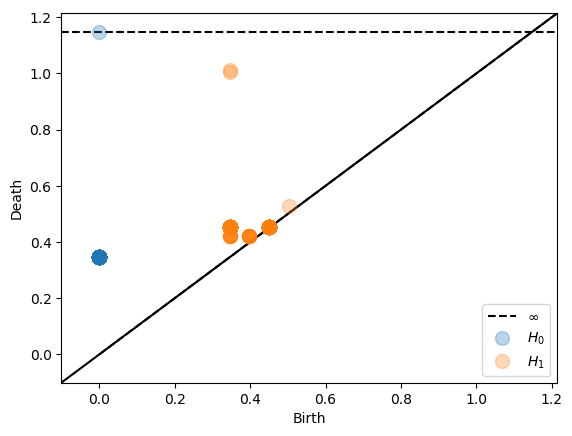
We start by calculating Čech persistent homology of a point cloud in 4-dimensional Euclidean space. First we import the relevant python packages and generate the sample data used for the examples below. The first data we use are 80 points on the Clifford torus. In order to calculate the persistent homology of a point cloud with an ambient Čech complex, we create a Persistence object. By default the plot_persistence method takes as input a dowker matrix X and returns the persistence diagram of the associated dowker nerve. Alternatively plot_persistence can be used with dissimilarity='ambient' to calculate ambient Čech complex. Information about the sizes of the nerves can be obtained by the cardinality_information method.

%matplotlib inline
from dowker_homology.datasets import clifford_torus
from dowker_homology.persistence import Persistence
# generate data
coords = clifford_torus(80)
# calculate and plot persistent homology
pers = Persistence(dissimilarity='ambient')
pers.plot_persistence(X=coords, alpha=0.3, show=True)

The parameter coeff_field is the characteristic p of the coefficient field Z/pZ for computing homology. See gudhi for more information. The max_simplex_size parameter helps by giving an error if the resulting nerve is very large and calculations will take a long time. Then the options are to either set max_simplex_size higher and expect some waiting time or to change the interleaving parameters so that calculations finish after reasonably short times.

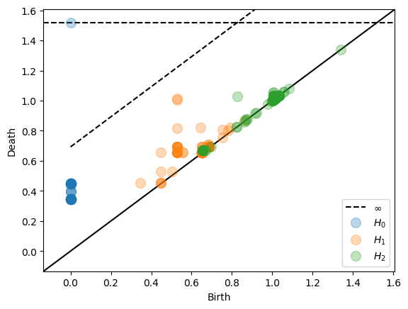
Two important optional parameters for Persistence objects are the maximal homology dimension dimension and the number n_samples of vertices in the nerve. We use a farthest point sampling to reduce the number of vertices.

from dowker_homology.datasets import clifford_torus
from dowker_homology.persistence import Persistence
# generate data
coords = clifford_torus(80)
# calculate and plot persistent homology
pers = Persistence(dimension=2,
                   n_samples=40,
                   dissimilarity='ambient')
pers.plot_persistence(X=coords, alpha=0.3, show=True)

After plotting the persistence diagram the Persistence object contains the variable homology, a numpy array with three columns. The first column gives homological dimension. The second column gives birth. The third column gives death.

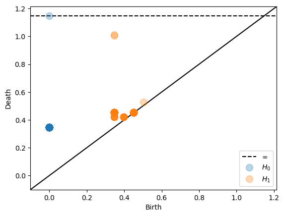
Intrinsic Čech complex

Instead of the ambient Čech complex we can compute the intrinsic Čech complex. For the intrinsic Čech complex we can specify all metrics accepted by scipy.spatial.distance.cdist or if the metric is precomputed we can specify 'metric'.

from dowker_homology.datasets import clifford_torus
from dowker_homology.persistence import Persistence
# generate data
coords = clifford_torus(80)
# calculate and plot persistent homology
pers = Persistence(dissimilarity='euclidean')
pers.plot_persistence(X=coords, alpha=0.3, show=True)

Alpha complexes

For eucliden point clouds in low dimension the alpha complex is the most efficient complex computing Čech homology. This complex can be used by setting dissimilarity='alpha'. On a technical note, we have actually implemented the Delaunay-Čech complex.

from dowker_homology.datasets import clifford_torus
from dowker_homology.persistence import Persistence
# generate data
coords = clifford_torus(80)
# calculate and plot persistent homology
pers = Persistence(dissimilarity='alpha')
pers.plot_persistence(X=coords, alpha=0.3, show=True)

Sparse Dowker Nerves

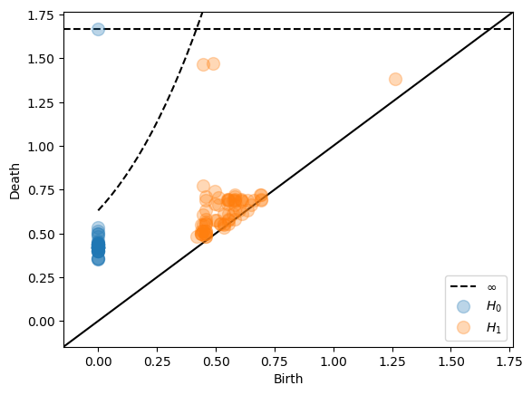
The sparse version of persistent homology from Example 5.6 in Sparse Filtered Nerves is interleaved with Čech persistent homology. The easiest way to use it is to specify the additive and multiplicative interleaving constants.

from dowker_homology.datasets import clifford_torus
from dowker_homology.persistence import Persistence
# generate data
coords = clifford_torus(80)
# calculate and plot persistent homology
pers = Persistence(dissimilarity='ambient',
                   additive_interleaving=0.1,
                   multiplicative_interleaving=1.5)
pers.plot_persistence(X=coords, alpha=0.3, show=True)

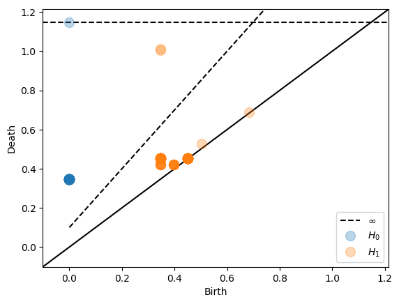
Note that there is a dashed interleaving line in addition to the top dashed line indicating infinity. The interleaving guarantees that all points above this interleaving line will be present in the original persistence diagram as well.

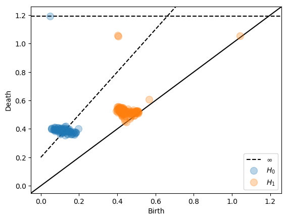
We can also sparsify the intrinsic Čech complex.

from dowker_homology.datasets import clifford_torus
from dowker_homology.persistence import Persistence
# generate data
coords = clifford_torus(80)
# calculate and plot persistent homology
pers = Persistence(dissimilarity='euclidean',
                   additive_interleaving=0.2,
                   multiplicative_interleaving=1.5)
pers.plot_persistence(X=coords, alpha=0.3, show=True)

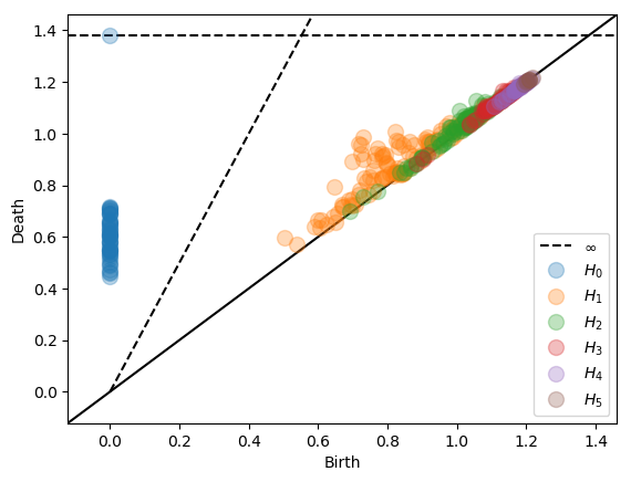
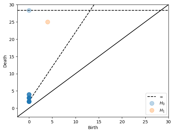
For data of high dimension we are able to reduce the size of the nerve drastically by using a multiplicative interleaving. We illustrate this on a dataset consisting of random data in 16 dimensional euclidean space.

import numpy as np
import urllib.request
from io import BytesIO
from dowker_homology.datasets import clifford_torus
from dowker_homology.persistence import Persistence

# Download data and transform to numpy array
url = ('https://raw.githubusercontent.com/' +
       'n-otter/PH-roadmap/master/data_sets/' +
       'roadmap_datasets_point_cloud/random_' +
       'point_cloud_50_16_.txt')

response = urllib.request.urlopen(url)
data = response.read()
text = data.decode('utf-8')
coords = np.genfromtxt(BytesIO(data), delimiter=" ")

# calculate and plot persistent homology
pers = Persistence(dimension=7,
                   dissimilarity='ambient',
                   multiplicative_interleaving=2.5)
pers.plot_persistence(X=coords, alpha=0.3, show=True)

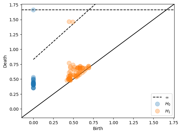
Subspace sparsification

In the introduction of Sparse Filtered Nerves we mention the additive interleaving of subspaces with the Hausdorff distance. This additive part can be specified using either the resolution or the n_samples parameters. If there is no other interleaving, the resolution parameter is the intersect of the interleaving line with the y-axis. The parameter n_samples specifies how many points to sample in a farthest point sampling. It is convenient, because computing time is low for few points. It can also be used to find an appropriate value for the resolution parameter. For a general alpha-interleaving the total interleaving is alpha(t + resolution). Here we use the clifford torus with 2000 points and specify n_samples to be 50.

from dowker_homology.datasets import clifford_torus
from dowker_homology.persistence import Persistence
# generate data
coords = clifford_torus(2000)
# calculate and plot persistent homology
pers = Persistence(dissimilarity='euclidean',
                   multiplicative_interleaving=1.2,
                   n_samples=50)
pers.plot_persistence(X=coords, alpha=0.3, show=True)

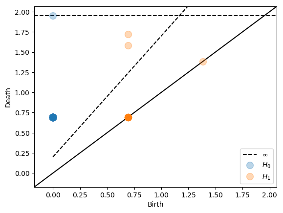
General interleavings

We can also specify interleavings with an arbitrary translation function α(t). Note that there are no automated checks of the correctness of α(t) so it is the users responsability to make sure that it is indeed a translation function. The following example gives the same result as the example with multiplicative interleaving of 2.5 and an additive interleaving of 0.5.

from dowker_homology.datasets import clifford_torus
from dowker_homology.persistence import Persistence
# generate data
coords = clifford_torus(2000)
# specify translation function
def translation(time):
    return 2.5 * time + 0.5
# calculate and plot persistent homology
pers = Persistence(dissimilarity='euclidean',
                   translation_function=translation,
                   n_samples=50)
pers.plot_persistence(X=coords, alpha=0.3, show=True)

More complex translation functions can also be specified.

from dowker_homology.datasets import clifford_torus
from dowker_homology.persistence import Persistence
# generate data
coords = clifford_torus(2000)
# specify translation function
def translation(time):
    return pow(time, 3) + 0.3
# calculate and plot persistent homology
pers = Persistence(dissimilarity='euclidean',
                   translation_function=translation,
                   n_samples=50)
pers.plot_persistence(X=coords, alpha=0.3, show=True)

Dowker dissimilarities

The package dowker_homology can compute persistent homology for Dowker dissimilarities defined on finite sets.

Below we compute persistent homology of the dowker nerve of the function X × G → [0, ∞] specifying the distance between a point x in the Clifford torus X and a point g in a grid G containing X.

from scipy.spatial.distance import cdist
from dowker_homology.datasets import clifford_torus
from dowker_homology.persistence import Persistence
# generate data
coords = clifford_torus(80)
grid = np.stack(np.meshgrid(
  np.linspace(-1, 1, 10),
  np.linspace(-1, 1, 10),
  np.linspace(-1, 1, 10),
  np.linspace(-1, 1, 10)), -1).reshape(-1, 4)
dowker_dissimilarity = cdist(coords, grid)
# calculate and plot persistent homology
pers = Persistence(dissimilarity='dowker',
                   additive_interleaving=0.2,
                   multiplicative_interleaving=1.5)
pers.plot_persistence(X=dowker_dissimilarity,
                      alpha=0.3, show=True)

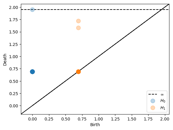
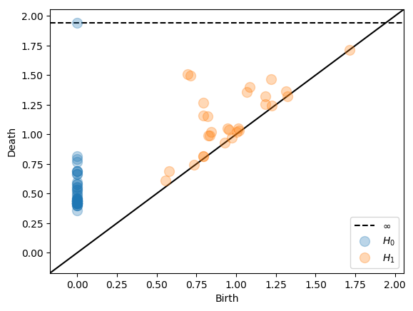
Inspired by the persnet software, we compute Dowker homology of cyclic networks.

from networkx import cycle_graph
from dowker_homology.datasets import clifford_torus
from dowker_homology.persistence import Persistence
# generate data
graph = cycle_graph(100)
# calculate and plot persistent homology
pers = Persistence(dissimilarity='dowker',
                   additive_interleaving=2.0,
                   multiplicative_interleaving=2.0)
pers.plot_persistence(X=graph, alpha=0.3, show=True)

We next compute the intrinsic Čech complex directly from the distance matrix. In order to take advantage of the triangle inequality, we use dissimilarity=‘metric’.

from scipy.spatial.distance import cdist
from dowker_homology.datasets import clifford_torus
from dowker_homology.persistence import Persistence
# generate data
coords = clifford_torus(80)
# calculate and plot persistent homology
pers = Persistence(dissimilarity='metric',
                   additive_interleaving=0.2,
                   multiplicative_interleaving=1.5)
pers.plot_persistence(X=cdist(coords, coords),
                      alpha=0.3, show=True)

Alternative restrictions and truncations

So far we have not talked about how we truncate and sparsify the Dowker dissimilarity. Usually the default methods truncation_method='dowker' and restriction_method='dowker' work best. Other methods are provided as a reference to compare the different strategies and examples in Sparse Dowker Nerves and Sparse Filtered Nerves.

We have implemented truncation methods described by Cavanna, Jahanseir and Sheehy in A Geometric Perspective on Sparse Filtrations and Definition 6 in Sparse Dowker Nerves, which we termed 'Sheehy' and the canonical truncation method described in Sparse Dowker Nerves, here called 'Canonical'.

The two restriction methods implemented here come from Sparse Dowker Nerves and are termed 'Sheehy' for the method described in Proposition 1 and 'Parent' for the method described in Definition 8. Note that the 'Sheehy' restriction is only compatible with the 'Sheehy' truncation.

Below we show a short simulation study to compare all different restriction and truncation methods.

import numpy as np
import pandas as pd
from scipy.spatial.distance import cdist
from dowker_homology.datasets import clifford_torus
from dowker_homology.persistence import Persistence

# generate data
coords = clifford_torus(40)
dists = cdist(coords, coords, metric='euclidean')

# set parameters
params = {'dimension': 1,
          'multiplicative_interleaving': 2.5,
          'dissimilarity': 'metric'}

# initiate persistence objects
pers_no_no = Persistence(truncation_method='no_truncation',
                         restriction_method='no_restriction',
                         **params)
pers_no_dowker = Persistence(truncation_method='no_truncation',
                             restriction_method='dowker',
                             **params)
pers_no_parent = Persistence(truncation_method='no_truncation',
                             restriction_method='Parent',
                             **params)

pers_dowker_no = Persistence(truncation_method='dowker',
                             restriction_method='no_restriction',
                             **params)
pers_dowker_dowker = Persistence(truncation_method='dowker',
                                 restriction_method='dowker',
                                 **params)
pers_dowker_parent = Persistence(truncation_method='dowker',
                                 restriction_method='Parent',
                                 **params)

pers_canonical_no = Persistence(truncation_method='Canonical',
                                restriction_method='no_restriction',
                                **params)
pers_canonical_dowker = Persistence(truncation_method='Canonical',
                                    restriction_method='dowker',
                                    **params)
pers_canonical_parent = Persistence(truncation_method='Canonical',
                                    restriction_method='Parent',
                                    **params)

pers_sheehy_no = Persistence(truncation_method='Sheehy',
                             restriction_method='no_restriction',
                             **params)
pers_sheehy_dowker = Persistence(truncation_method='Sheehy',
                                 restriction_method='dowker',
                                 **params)
pers_sheehy_parent = Persistence(truncation_method='Sheehy',
                                 restriction_method='Parent',
                                 **params)
pers_sheehy_sheehy = Persistence(truncation_method='Sheehy',
                                 restriction_method='Sheehy',
                                 **params)

# calculate persistent homology
pers_no_no.persistent_homology(X=dists)
pers_no_dowker.persistent_homology(X=dists)
pers_no_parent.persistent_homology(X=dists)

pers_dowker_no.persistent_homology(X=dists)
pers_dowker_dowker.persistent_homology(X=dists)
pers_dowker_parent.persistent_homology(X=dists)

pers_canonical_no.persistent_homology(X=dists)
pers_canonical_dowker.persistent_homology(X=dists)
pers_canonical_parent.persistent_homology(X=dists)

pers_sheehy_no.persistent_homology(X=dists)
pers_sheehy_dowker.persistent_homology(X=dists)
pers_sheehy_parent.persistent_homology(X=dists)
pers_sheehy_sheehy.persistent_homology(X=dists)

# setup the summary function
def summarize_one(pers):
    cardinality = pers.cardinality_information(verbose = False)
    return pd.DataFrame(
        {'truncation': [pers.truncation_method],
         'restriction': [pers.restriction_method],
         'unreduced': [cardinality.get('unreduced_cardinality', np.nan)],
         'reduced': [cardinality.get('reduced_cardinality', np.nan)]},
        columns = ['truncation', 'restriction', 'unreduced', 'reduced'])

def summarize_sizes(*args):
    return pd.concat([summarize_one(arg) for arg in args])

# sizes
summarize_sizes(pers_no_no,
                pers_no_dowker,
                pers_no_parent,
                pers_dowker_no,
                pers_dowker_dowker,
                pers_dowker_parent,
                pers_canonical_no,
                pers_canonical_dowker,
                pers_canonical_parent,
                pers_sheehy_no,
                pers_sheehy_dowker,
                pers_sheehy_parent,
                pers_sheehy_sheehy)

	truncation	restriction	unreduced	reduced
0	no_truncation	no_restriction	10700.0	NaN
0	no_truncation	dowker	10700.0	10700.0
0	no_truncation	Parent	10700.0	10700.0
0	dowker	no_restriction	10700.0	10700.0
0	dowker	dowker	10700.0	140.0
0	dowker	Parent	10700.0	2435.0
0	Canonical	no_restriction	10700.0	10700.0
0	Canonical	dowker	10700.0	333.0
0	Canonical	Parent	10700.0	1082.0
0	Sheehy	no_restriction	10700.0	5119.0
0	Sheehy	dowker	10700.0	3944.0
0	Sheehy	Parent	10700.0	3644.0
0	Sheehy	Sheehy	10700.0	4918.0

Persistence in pipelines

We also provide a seperate class PersistenceTransformer that can be used to integrate persistence in a sklearn pipline. The main method fit returns the persistence diagrams that can be used for example in the persim package. The example below shows how a PersistenceTransformer can be used to predict the parameters of a linked twist map. Note that this is a toy example and larger datasets are needed to get reasonable accuracies.

import numpy as np
from sklearn.base import BaseEstimator
from sklearn.pipeline import Pipeline
from sklearn.ensemble import RandomForestClassifier
from sklearn.model_selection import train_test_split
from sklearn.metrics import accuracy_score
from persim import PersImage
from dowker_homology.persistence import PersistenceTransformer
from dowker_homology.datasets import linked_twist_map

# generate data
np.random.seed(1)
N = 100
k = 5
r_values = np.repeat([2.0, 3.5, 4.0, 4.1, 4.3], k)
labels = r_values.astype('str')
data = [linked_twist_map(N=N, r=r) for r in r_values]

# train test split
(X_train, X_test, y_train, y_test) = train_test_split(
    data, labels, test_size=0.33, random_state=42)

# some pipeline steps
class PrepareDiagrams(BaseEstimator):
    def __init__(self):
        pass
    def fit(self, X, y=None):
        pass
    def transform(self, X, y=None):
        dgm_result_list = list()
        for dgms in X:
            dgm_result = list()
            for dgm in dgms:
                dgm = dgm[np.isfinite(dgm[:, 1])]
                dgm_result.append(dgm)
            dgm_result_list.append(dgm_result)
        return dgm_result_list
    def fit_transform(self, X, y=None):
        return self.transform(X=X, y=y)

class PersistenceImage(BaseEstimator):
    def __init__(self, spread=1, pixels=[10, 10]):
        self.spread = spread
        self.pixels = pixels
        self.pim0 = PersImage(spread=self.spread,
                              pixels=self.pixels,
                              verbose=False)
        self.pim1 = PersImage(spread=self.spread,
                              pixels=self.pixels,
                              verbose=False)
    def fit(self, X, y=None):
        pass
    def transform(self, X, y=None):
        img_0d = self.pim0.transform([dgm[0] for dgm in X])
        img_1d = self.pim1.transform([dgm[1] for dgm in X])
        img = [np.hstack((im0, im1)) for im0, im1 in zip(img_0d, img_1d)]
        image_dta = np.vstack([np.hstack([im.ravel() for im in image])
                               for image in img])
        self.img_0d = img_0d
        self.img_1d = img_1d
        return image_dta
    def fit_transform(self, X, y=None):
        return self.transform(X=X, y=y)

# define pipeline
pers = PersistenceTransformer(
    dissimilarity='euclidean',
    multiplicative_interleaving=1.5)
prep = PrepareDiagrams()
pim = PersistenceImage(spread=1, pixels=[10,10])
rf = RandomForestClassifier(n_estimators=100)
pipe = Pipeline(steps=[('pers', pers),
                       ('prep', prep),
                       ('pim', pim),
                       ('rf', rf)])

# fit model
pipe.fit(X_train, y_train)

# predictions
y_pred = pipe.predict(X_test)

# accuracy
acc = accuracy_score(y_test, y_pred)
print('Accuracy: {0:.2f}'.format(acc))

Accuracy: 0.67